深度转视差代码

内参fx可以从镜头焦距F,sensor_width直接计算得到

import cv2
import numpy as np
import matplotlib.pyplot as plt


depth_l = np.load('stereo_pinhole/0000.npy')
depth_r = np.load('stereo_pinhole/0001.npy')
img_l = cv2.imread('stereo_pinhole/0000.png')
img_r = cv2.imread('stereo_pinhole/0001.png')


# ---------------------------
# 相机参数设置
f_mm = 1.93          # 焦距，单位 mm
sensor_width = 3.84  # 传感器宽度，单位 mm
B = 0.1              # 基线，单位 m (10 cm)

# 图像分辨率（以深度图尺寸为准）
img_h, img_w = depth_l.shape

# 计算水平内参 fx （单位：pixel）
fx = f_mm * (img_w / sensor_width)
print("Computed fx: {:.2f} pixels".format(fx))
# 例如，2560/3.84 ≈ 666.67，fx ≈ 1.93*666.67 ≈ 1287 pixels

# ---------------------------
# 计算视差图 disp_l
disp_l = np.zeros_like(depth_l, dtype=np.float32)
valid_mask = depth_l > 0  # 有效区域
# 对有效区域，按照公式：disp = fx * B / depth
disp_l[valid_mask] = fx * B / depth_l[valid_mask]
# 对无效区域（depth_l == -1），这里设为 0
disp_l[~valid_mask] = 0

# ---------------------------
# 使用视差对左图进行 warp 操作
# 建立图像网格
grid_x, grid_y = np.meshgrid(np.arange(img_w), np.arange(img_h))
# 由于公式 x_right = x_left - disp，
# remap 时 map_x 设定为左图的 x 坐标扣除视差即可生成“右图”像素位置
map_x = (grid_x + disp_l).astype(np.float32)
map_y = grid_y.astype(np.float32)

# 对 img_l 进行水平 warp，生成合成的右视图（synthetic right image）
# ! cv2.remap输入target的坐标在source的采样,所以map_x = (grid_x + disp_l).astype(np.float32)
img_r_syn = cv2.remap(img_l, map_x, map_y, interpolation=cv2.INTER_LINEAR, borderMode=cv2.BORDER_CONSTANT)

# ---------------------------
gray_syn = cv2.cvtColor(img_r_syn, cv2.COLOR_BGR2GRAY)
gray_r = cv2.cvtColor(img_r, cv2.COLOR_BGR2GRAY)

# Step 2: 使用 Canny 算法提取边缘
edges_syn = cv2.Canny(gray_syn, threshold1=50, threshold2=150)
edges_r = cv2.Canny(gray_r, threshold1=50, threshold2=150)

# Step 3: 创建空白的彩色边缘图用于显示
# 为方便观察，我们把提取的边缘上色：synthetic右图边缘设为红色，真实右图边缘设为绿色
edge_syn_color = np.zeros_like(img_r_syn)
edge_r_color = np.zeros_like(img_r)

# 在 BGR 色彩空间中，将 synthetic 边缘设为红色 (0,0,255)
edge_syn_color[edges_syn != 0] = [0, 0, 255]
# 将真实右图边缘设为绿色 (0,255,0)
edge_r_color[edges_r != 0] = [0, 255, 0]

# Step 4: 叠加两幅上色的边缘图，可以简单相加（注意像素值可能会溢出，但一般显示没有问题）
edge_overlay = cv2.addWeighted(edge_syn_color, 0.99, edge_r_color, 0.99, 0)

# Step 5: 将边缘叠加到真实右图上，便于直观查看对齐情况
img_r_overlay = cv2.addWeighted(img_r, 0.7, edge_overlay, 0.3, 0)

# 转换为灰度图
gray_syn = cv2.cvtColor(img_r_syn, cv2.COLOR_BGR2GRAY)
gray_r   = cv2.cvtColor(img_r, cv2.COLOR_BGR2GRAY)

# 提取边缘：参数可以根据需要调整
edges_syn = cv2.Canny(gray_syn, threshold1=50, threshold2=150)
edges_r   = cv2.Canny(gray_r, threshold1=50, threshold2=150)

# ---------------------------
# 定义有效区域掩码
# 假设 img_r_syn 中，非黑色区域（比如不为 [0,0,0]）为有效区域
# 这里以灰度图为例，假设有效区域像素值非零为有效（你也可以根据原始数据进行判断，比如根据 depth 有效性）
mask_valid = (cv2.cvtColor(img_r_syn, cv2.COLOR_BGR2GRAY) > 0)

# 将边缘图也限制在有效区域内
edges_syn_valid = np.zeros_like(edges_syn)
edges_r_valid   = np.zeros_like(edges_r)

edges_syn_valid[mask_valid] = edges_syn[mask_valid]
edges_r_valid[mask_valid]   = edges_r[mask_valid]

# ---------------------------
# 计算有效区域内边缘 IoU
# 将边缘二值化，确保只有 0 或 1
bin_edges_syn = (edges_syn_valid > 0).astype(np.uint8)
bin_edges_r   = (edges_r_valid > 0).astype(np.uint8)

intersection = np.logical_and(bin_edges_syn, bin_edges_r).sum()
union = np.logical_or(bin_edges_syn, bin_edges_r).sum()

if union > 0:
    edge_iou = intersection / union
else:
    edge_iou = 0

print("Edge IoU in valid region: {:.4f}".format(edge_iou))


# 展示结果
plt.figure(figsize=(15,5))

plt.subplot(2,3,1)
plt.title("Synthetic Right Edges (Red)")
plt.imshow(cv2.cvtColor(edge_syn_color, cv2.COLOR_BGR2RGB))
plt.axis('off')

plt.subplot(2,3,2)
plt.title("Real Right Edges (Green)")
plt.imshow(cv2.cvtColor(edge_r_color, cv2.COLOR_BGR2RGB))
plt.axis('off')

plt.subplot(2,3,3)
plt.title("Overlay of Edges (Red + Green)")
plt.imshow(cv2.cvtColor(edge_overlay, cv2.COLOR_BGR2RGB))
plt.axis('off')

plt.subplot(2,3,4)
plt.title("Real Left Image")
plt.imshow(cv2.cvtColor(img_l, cv2.COLOR_BGR2RGB))
plt.axis('off')

plt.subplot(2,3,5)
plt.title("Real Right Image")
plt.imshow(cv2.cvtColor(img_r, cv2.COLOR_BGR2RGB))
plt.axis('off')

plt.subplot(2,3,6)
plt.title("Synthetic Right Image")
plt.imshow(cv2.cvtColor(img_r_syn, cv2.COLOR_BGR2RGB))
plt.axis('off')

plt.tight_layout()
plt.show()
exit()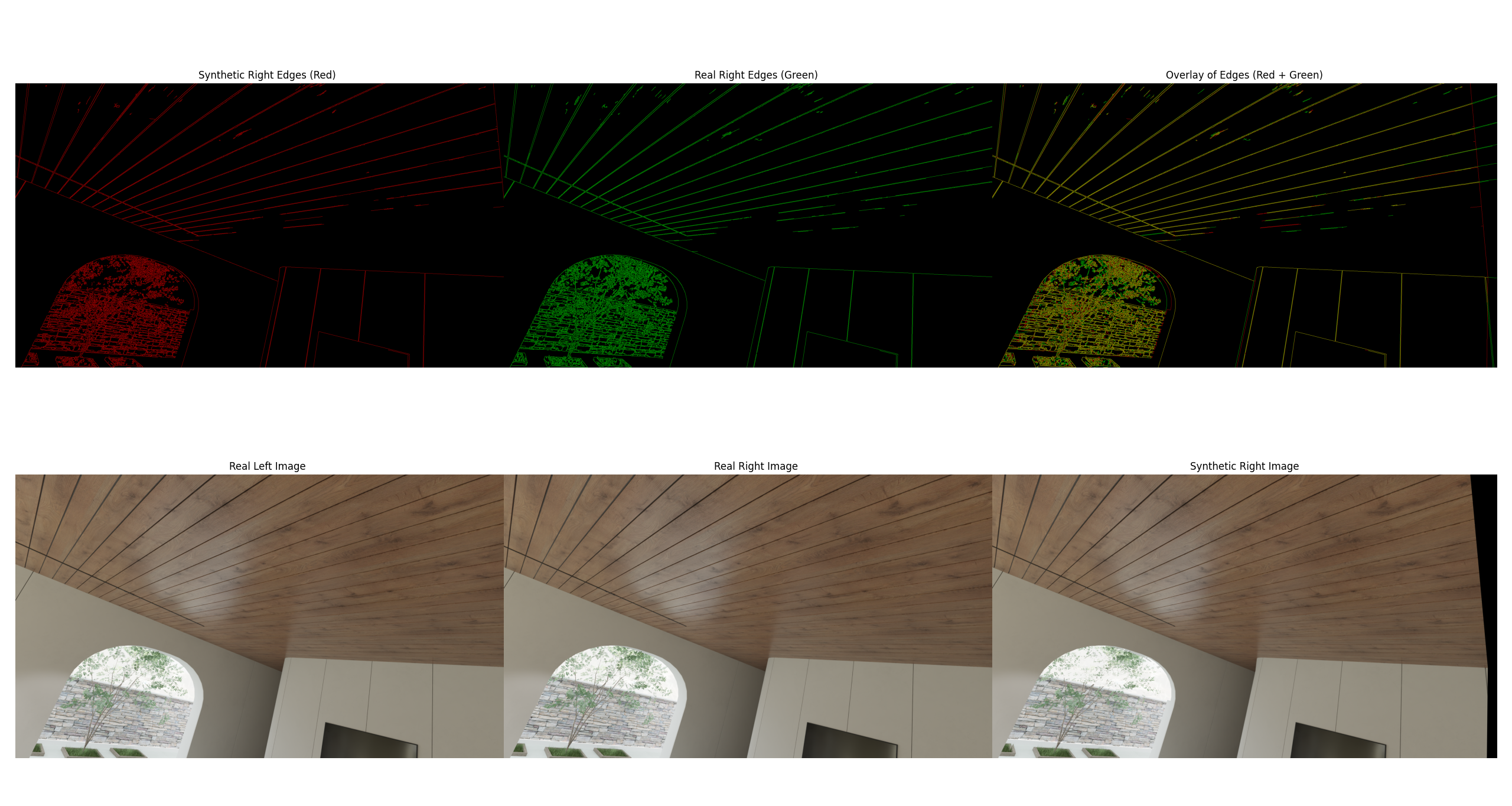

右上角的图显示左图+视差后与右图边缘特征高度重合,证明算出的视差是正确的.可以作为真值进行训练或测试.